Understanding TrainingPeaks Ramp Rate For Better Coaching
Understanding ramp rate will help you keep better track of your athletes’ Chronic Training Load and fatigue as you and your athletes gear up for racing season.
TrainingPeaks not so recently released WKO4. Many coaches’ minds were blown upon gazing at a dozen or so new ways of measuring our cycling metrics and analyzing our athletes’ efforts and fatigue. One of these new metrics is “ramp rate.” This metric is not any more or less important than Time to Exhaustion (TTE), Stamina or Functional Reserve Capacity (FRC) but it has a large importance in tracking Chronic Training Load (CTL), Training Stress Score В® (TSS В® ), and fatigue and, as this is the time of year for increased training load, and therefore increased ramp rate, this fatigue measure has heightened seasonal significance. If you are unfamiliar with these terms check out the TrainingPeaks glossary of terms page.
To define ramp rate we need to know what Training Stress Score (TSS) and Chronic Training Load (CTL) are. TSS is a stress score based on the fatigue a certain effort or ride will place on your body. TSS is defined by the Intensity Factor В® , which is Normalized Power В® as a fraction of threshold power, and duration of the effort or day’s ride. These TSS scores are added up day-by-day to make the average daily TSS, or Chronic Training Load.
So now that we have that under our belts, what is ramp rate? Defined by TrainingPeaks, “The ramp rate, expressed in TSS/day, shows daily rate of change (both positive or negative) that your CTL changes.”
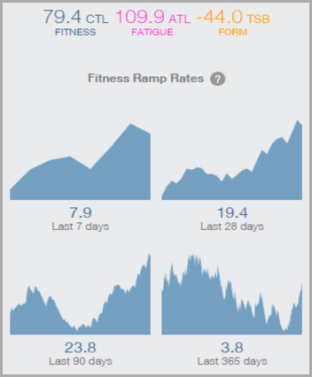
For Premium athletes on TrainingPeaks, under your Home tab on the web or in the Fitness Report in the mobile app, ramp rate is expressed in 7, 28, 90, and 365 day periods as seen below.
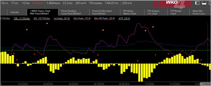
In WKO4 (below) the ramp rate is located on the very top in the Hero Bar. You can set your ramp rate constants and when the red “warning” color shows up depending on the “normal” client fatigue for each client.
When comparing WKO4 and TrainingPeaks (TP), make sure you are comparing the same data in both programs. You need all workouts to be in WKO from TP. Make sure your athlete’s history is correct or matching that on TP. WKO is based on the Set FTP (sFTP) not Modeled FTP (mFTP). TSS is calculated from sFTP so if there’s different data and different athlete history then the ramp rate will not be the same as TSS per day created CTL and ramp rate.
Since we know that with fatigue comes fitness, we expect to have a positive ramp rate to increase fitness. That’s pretty much the only solid assumption to the most frequent question of, “What should my ramp rate be?” Ramp rate may not be positive 100 percent of the time. We expect to see negative ramp rates during longer rest periods. Other than that, each athlete can expect to have different ramp rates.
The TP ramp rate example above is from a client in Colorado that had very mild fall weather,В which drove us to give him a large block of training. As you can imagine with such a large ramp rate and jump in CTL, he is pretty tired right now but, with some recovery, he will come back a monster. Another factor is that, toward the end of the summer, this athlete’s race season ended a bit early. He had fewer days with high TSS and thus lost TSS per day, resulting in a negative ramp rate, while losing CTL or losing average TSS per day. As he started this ramp rate at a lower TSS per day, he can have a steeper short term ramp rate.
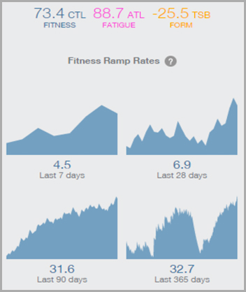
The main point is that every rider’s ramp rate is a function of how they are gaining fatigue in that moment where their CTL started off and that rider’s ability to hold fatigue. You will also see a large ramp rate with someone who is new to power and starts at zero TSS per day. Obviously every day with a TSS score after 0 will have a positive ramp rate. Here is a client who just got a power meter in August. We expect to see a large ramp rate until he gets to a point where an increase in CTL is not raising his average CTL per day making his ramp rate so steep.
The opposite example to the “new to power” athlete is the athlete that has years of power data. This specific long-term power athlete never really loses CTL year to year. This rider is still being built with specific workouts at different time per year for their events and goals but holding a constant Chronic Training Load will make an increased ramp rate or a jump in CTL a challenge. On one hand it seems like diminishing returns. You will have elite riders that carry CTL see less gains in general, but even riders newer to cycling that are seeing larger gains will have a hard time increasing their ramp rate if they carry a large CTL for an entire year. These different comparisons should key you into what type of rider they are, how they carry fatigue and then how much resting to building they should be doing.

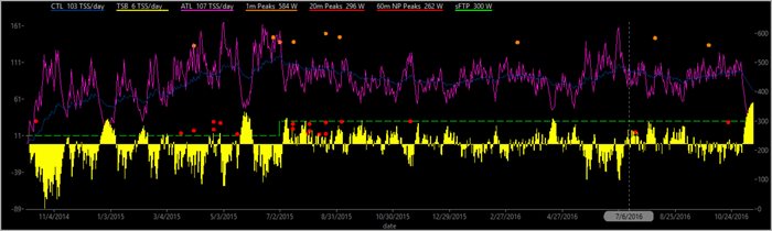
This athlete has a set amount of time to train. He can’t get a huge ramp rate but, in the same breath, he does not need large rest periods. After three years of data, I know from ramp rate when we are really pushing versus when we are sustainable. For this athlete, the difference in ramp rate is very small between overreaching and rested. This is another example of how each athlete needs customized training and tracking.
There are a few things to watch out for that may skew ramp rate. We need good data and good Functional Threshold Power (FTP) settings. Beside the fact that having wrong or unset FTP history in WKO4 will make everything incorrect, it will also skew TSS and everything calculated downstream. If the FTP is set too high, your IF will read low for the day. Since TSS per day makes CTL, an FTP estimation too high will skew TSS down, CTL down, and then ramp rate will be low. This will drive you as a coach to push the athlete to greater fatigue, maybe even overtraining just from analyzing bad data. As coaches we need good data, accurate power meters, and accurate FTP or field testing data to make everything downstream correct. Since 100-percent correct data does not happen, a good coach needs to be able to pick out right and wrong data and use the tools at hand to find bad patches and deal with them accordingly. Sometimes it takes hours to pinpoint a bad file with major spikes or bad calibration but that file has to be corrected if we want to trust overall metrics computed by WKO4 and TrainingPeaks.
One other thing that catches people and coaches off guard is the idea of accumulating fatigue from outside factors. If, for example, the mental fatigue that this election caused on my brain was trackable in a TrainingPeaks metric, that was put into CTL, my ramp rate would be through the roof. There’s no way to track some things but they should be tracked in some way in TP or on the side to make sure the rider is not overreaching despite ramp rate being low or stagnant. Some examples are running workouts, non-power but HR and TSS trackable workouts, and all the workouts that create fatigue like hiking or snowshoeing.
Once everything is correct we can use ramp rate as one of the new metrics for fatigue tracking, tapers, overreaching prevention and just solid, fundamental data-driven coaching.
Learn more about WKO4 features and how-to videos or try it free for 14 days.
Источник
Ramp Rate
Related terms:
Download as PDF
About this page
Flexible active power control of PV systems
6.5 Power ramp-rate control (PRRC)
The power ramp-rate control (PRRC) strategy is employed to limit the fluctuation rate in the PV output power under dynamically changing irradiance conditions (e.g., passing clouds). In this operation mode, the PV output power is controlled in a ramp-changing manner in order to limit its change rate to a certain value R r ⁎ [41] . Clearly, to achieve the PRRC, the change rate of the PV output power R(t) should be continuously measured, which can be calculated as
where Δ ppv is the power difference measured in the time period of Δt. Notably, the measuring window (i.e., Δt ) of the ramp rate can also affect the performance of the PRRC strategy. This is mainly because the operating point of the PV system usually oscillates in steady state due to the MPP searching (e.g., the P&O MPPT algorithm). Therefore, the measured ramp rate of the PV power will not be zero even under a constant solar irradiance condition. In prior-art solutions, a moving average or a low-pass filter is usually employed to reduce the power oscillation [14] , [42] and to improve the measurement. In this regard, the ramp-rate measurement is a challenge issue when implementing the PRRC.
The measured ramp rate calculated by Eq. (6.12) is the key to determining the operating mode of the PV system. More specifically, as long as the ramp rate of the PV power R(t) is below the ramp-rate limit R r ⁎ (e.g., under slow changing irradiance conditions), the MPPT operation can be employed, and the PV system delivers the maximum available power to the grid. This is demonstrated by the operation trajectory from A to B in the PV array characteristic in Fig. 6.26 . However, once the measured ramp rate exceeds the limit, the PV output power should be reduced from the maximum available value (e.g., power curtailment) in a way to lower the change rate and then follow the ramp-rate profile. This can be achieved by perturbing the operating point of the PV system away from the MPP, as it is illustrated by the operating trajectory from B to C in Fig. 6.26 . In this operation, the PV system will operate in the PLC mode with a dynamically changing power limit calculated according to the ramp rate. The PV voltage reference with the PRRC can be summarized as

Fig. 6.26 . Operational principle of the power ramp-rate control (PRRC) algorithm: MPPT mode (A → B) and PRRC mode (B → C), where R1 = (Pmpp1 − Pmpp2)/t1 and R2 = (Pmpp2 − Pmpp3)/t2 are the PV power ramp rates and R r ⁎ is the ramp-rate limit.
with v mpp ⁎ being the reference voltage from an MPPT algorithm (e.g., P&O MPPT) and vstep is the perturbation step size.
The performance of the PRRC strategy is demonstrated by employing two trapezoidal solar irradiance profiles with different slopes to emulate different changing solar irradiance conditions. First, the PRRC strategy is demonstrated with the slow changing solar irradiance condition in Fig. 6.27 A, where two different ramp-rate limits of R r ⁎ = 10 and 20 W/s are employed. It can be seen from Fig. 6.27 A that the PV power is in the ramp-changing manner when the solar irradiance increases (i.e., the PV power increases). The corresponding ramp rate is measured in Fig. 6.28 A, indicating that the PRRC strategy can limit the ramp rate of the PV power. Similar performance can also be observed in the case of fast changing solar irradiance condition in Fig. 6.27 B. In this case, it is more challenging for the PRRC strategy to limit the ramp rate, where it can be seen in Fig. 6.28 B that the instantaneous power ramp rate R(t) exceeds the limit temporarily during a transient (e.g., rapid increase of solar irradiance level). Nonetheless, the change rate can still be limited with the PRRC strategy.

Fig. 6.27 . Performance of the PRRC strategy with different ramp-rate limits under: (A) a slowly changing and (B) a fast changing irradiance condition.

Fig. 6.28 . Measured ramp rate of the PRRC strategy with different ramp-rate limits under (A) a slowly changing and (B) a fast changing irradiance condition.
Furthermore, the test with two daily real-field solar irradiance profiles (a clear day and a cloudy day) is also carried out (with an acceleration from 24 h to 24 min) where the ramp-rate limit of R r ⁎ = 10 W / s is adopted. The experimental results are shown in Figs. 6.29 and 6.30 . Under the clear-day condition, the solar irradiance changes with a slow and smooth transition, as it can be seen from the available power in Fig. 6.29 A. The ramp rate of the PV power can be accurately controlled with the PRRC strategy as it can be observed from the PV output power and the corresponding ramp rate in Figs. 6.29 A and 6.30 A, respectively. However, when the cloudy day profile is adopted, the ramp rate is difficult to control, as shown in Fig. 6.29 B. It can be seen that although the PV output power is controlled in a ramp-changing manner, it presents variations, as observed in Fig. 6.30 B. Notably, there is a short period, where the ramp-rate limit is violated due to the very fast dynamics in the solar irradiance. In that case, the algorithm requires a certain iteration (sample periods) to reduce the PV power following the ramp-rate demand. Nevertheless, the results have demonstrated the effectiveness of the PRRC strategy that can be applied to various operating conditions. Moreover, it is worth to be mentioned that the PRRC algorithm can only reduce the ramp rate during the increasing solar irradiance condition (i.e., power ramp up). During the fast decreasing in the solar irradiance, the PV system needs to provide extra power (higher than the available power) in order to maintain the ramp-down rate, which fundamentally cannot be achieved by the power curtailment (i.e., the FPPT control). A possible solution to this situation is to cooperate with the forecasting method to predict the ramp-down incident and thus reduce the PV power slightly before it occurs as proposed in [43] . Clearly, the above experimental tests verified that the ramp-up rate of the PV power could be limited when the PRRC is enabled.

Fig. 6.29 . Performance of the PRRC strategy with the ramp-rate limit of 10 W/s under two daily operation profiles: (A) a clear day and (B) a cloudy day.

Fig. 6.30 . Measured ramp rate of the PRRC strategy with the ramp-rate limit of 10 W/s under two daily operation profiles: (A) a clear day and (B) a cloudy day.
Источник