Chia plotter usage best settings

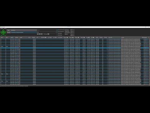
GUI Tool for beginners and experts to Monitor and Analyse Chia Plotting log files, show health and progress of running plots and estimated time to completion. No setup, configuration or installation of python or whatever required. Just install and enjoy.

Monitor Progress of running plots
Show estimated time to completion based on your already finished plots best matching your current plot config
Monitor Health of plotting processes
Already compatible with madMAx43v3r/chia-plotter (currently getting improved)
Compatible with all plotters and plotting managers that use or are based on the official chia plotter (see Troubleshooting if something does not work from the get go)
Show important information from log file in easy to read table
Multiple folders with log files supported (multiple plotting rigs, anyone?)
Multiple plots per log file supported (plot create —num n)
Export of readable or raw data to Json, Yaml and CSV

See Chia Plot Status in action:

On Upside Down Crypto (YouTube):

On Patro TV (YouTube):

Chia Plot Status observes the log folders you give it to monitor which can be local or connected via network. By this it supports monitoring multiple plotting rigs as you can access them on your desktop even if your plotting rigs are headless. It regulary checks for new Log files in those folders and analyses them.

On basis of finished plots it builds a local statistic (on your machine, no data is send anywhere or pulled from any cloud) and uses them to calculate ETA / time remaining and warning thresholds for the Health of your plotting processes.

Working with many distributed plotting rigs

Recommended way: Use sshfs (with sshfs-win for Windows) to securely mount the log dirs of your plotting rigs on your desktop via highly encrypted network connection, where it is your desktop that initiates the mount. This can be set up so that the desktop can only access the log dirs and only has read access. Even if you use remote plotting rigs that you access over the internet this is the most secure way and you most likely access your remote servers via ssh already.

Other Options: Mount the log folders of all rigs as network shares (via samba on linux) if all your plotting rigs are in the local network or connected via VPN. Another way would be to make a cronjob on your plotting rigs that uses scp or rsync in append mode to copy the log dir to your desktop where you run Chia Plot Status, but if you can manage to set this up you should set up sshfs instead. Last, least preferred option: collect them with cloud apps like Google Drive (Chia Plot Status does not talk to any cloud services for you, you have to install those apps and mount your log folders in them yourself if you want to use them).

Best Practice:

Only delete log files of finished plots if your hardware or the way you plot has significantly changed. Chia Plot Status uses finished plots to calculate ETA/Time Remaining as well as warning/error thresholds. If you delete finished log files the quality of those values decreases significantly.
Use SSHFS to access the log directories of your plotting rigs
Each plotting rig should have its own log folder, so they don’t mix and mess up estimates and warning thresholds for each other.
Always log locally. If you log directly to a network share / NAS your plotting processes will crash if the connection becomes flaky. Prefer connecting your host machine (which runs Chia Plot Status) to networkshares on the plotting rigs, not the other way around.

There are multiple attack vectors to consider:

1. The possibility that the core developer (me) is or becomes malicious

There is a saying: Where is a money trail, there is a way to sue/prosecute someone.

Chia Plot Status has buttons to donate via paypal both in the application itself and on the website.

Should the core developer (me) turn malicious, people could easily sue the core developer (me) and by that get the necessary details as in full name, address and day of birth, IBAN/Bic, everything from paypal.

If the core developer (me) becomes malicious this would be basically a how to get imprisoned speedrun (any %)

Even if you think you would not sue the core developer as he (me) might sit in a different country (germany), someone will as the Chia Plot Status Github Repository has between 2k to 4k visits daily and currently 24k downloads.

This should be more than enough to deter the core developer (me) from doing anything malicious.

2. The core developer (me) merges a pull request (code changes made by someone else) which contains malicious code without noticing

As seen on https://github.com/grayfallstown/Chia-Plot-Status/graphs/contributors there is only one other person who contributed a pull request so far and that wasn’t code but a documentation change.

The core developer (me) will check each pull request before merging as he (me) would have to run the code himself to check if the application works properly after merging that pull request and by that he (I) would get attacked by any malicious code that was contained in that pull request.

3. External Dependencies (as in libraries / code written by someone else) the application uses to do certain things (like to create the graphical user interface) become malicious.

Well, this is a tough one as even the core developer (me) has very little means to check external binaries for malicious code. The core developer (me) and every other developer using those libraries will get attacked by any malicious code in those libraries before they (we) distribute a new version of their (our) software containing that library to the users of their (our) softwares, as they (we) generally test their (our) applications before each release.

The core developer (me) takes the following precautions to mitigate that risk:

External dependencies are kept at a minimum to reduce this attack vector (chia-blockchain devs do the same)

Every release build is build on the same system and previously downloaded dependencies are never deleted/redownloaded. This prevents pulling in malicious code if the external dependency version used gets replaced with malicious code. But it also prevents reproducible builds that everyone can follow and reproduce step by step on their system, if the external dependency version actually does get changed. Well, this should raise concern anyway and in any case.

Updating Dependencies (external libraries / code written by someone else) is delayed (possibly indefinitely) until an update is required to implement a feature or to fix a bug. This gives anti virus providers time to determine if that library version is malicious, which would prevent an update.

Windows: Download latest version You will get a blue warning saying this was published by an unknown developer.

Linux: First install dotnet 5.0 SDK, then either the Chia Plot Status deb or rpm package depending on your linux distribution (deb for ubuntu)

For Mac you currently have to build it.

Getting Log Files from PowerShell

The last part with 2>&1 | % ToString | Tee-Object writes the log to the PowerShell and to a file with a unique name for each plotting process.

Getting Log Files from madMAx43v3r/chia-plotter

Источник

Chia plotting improvements in version 1.04

Download version 1.04 at Chia.net, official release notes

The Chia team is delivering a significant improvement to the plotter in version 1.04. The notable changes include a 26% reduction in memory resources required per plotting process and a 28% reduction in temporary storage space. The net result of this for many people will mean a significant boost in plotting output in TB/day on the same system! For new plotting system builders, this will mean different ratios of compute, memory, and storage.

Here is a quick example of some of the gains I saw in the version 1.04 beta…I will be testing a lot more systems in the coming weeks.

Example of real plotting improvements

System	change	Version 1.03	Version 1.04
NUC	5 → 6 processes	1.31TiB or 1.44TB per day	1.62TiB or 1.78TB per day
Intel Server System R2308WFTZSR	27 → 46 processes	6.77TiB or 7.44TB per day	9.16TiB or 10TB a day
Budget build, Z490	3TB → 2TB temp space (reduction $100-200)	3TB per day	3TB per day

New Temporary Space and Memory Requirements in 1.04

K-value	DRAM (MiB)	Temp Space (GiB)	Temp Space (GB)
32	3389	239	256.6
33	7400	512	550
34	14800	1041	1118
35	29600	2175	2335

Old Requirements in 1.03 and previous

K-value	DRAM (MiB)	Temp Space (GiB)	Temp Space (GB)
32	4608	332	356
33	9216	589	632
34	18432	1177	1264
35	36864	2355	2529

Example systems and new build options

System	Cost	CPU cores	DRAM (GiB)	Temp (GB)	SSD	Expected TB/day
Value desktop	$400	4	13.2	1024	1TB	1-2
Desktop	$700	6	20	1536	2x 800GB or 1x 1.6TB	2-3
Desktop	$900	8	26.5	2048	2x 1TB, 1x 2TB (stagger)	3-4
High-end desktop	$2000	12	39.7	3072	2x 1.6TB	4.5
High-end desktop	$3000	16	53	4096	5x 960GB	5-6
Server	$4000	32	106	8192	3x 3.2TB	8-10

What about staggering?

Staggering, or delaying the start of the following plotting process to start, can help maximize compute (CPU), memory (DRAM), and disk (temp space) utilization because different phases of the plotting process require different amounts of these resources. The main advantage of staggering in mid-range desktop systems with eight cores was squeezing eight processes into 32GB of DDR4 without having processes swap (slowdown) or getting killed (not enough memory). This speeds up the completion times of the phase1. The memory reduction mostly came from the fact that phase2 and phase3 of the plotting process were the most memory-intensive; ensuring that all the processes weren’t in this phase simultaneously meant better sharing of memory resources over time. There was a secondary effect of staggering of not thrashing the destination disk with multiple file copies from the second temporary directory (-2) to the final destination directory (-d) simultaneously. If a user only uses a single drive, this is a big deal because hard disk drive bandwidth is

100-275MB/s, depending on how full the disk is, and will delay the start of the following process while using an n value higher than 1. We will have to explore how the new 1.04 plotter changes staggering benefits in the coming weeks after the 1.04 release.

What about hyperthreading?

Another area to explore in 1.04 with running more processes than physical hardware CPU cores is typically 2x the number of CPU threads to physical cores due to a feature called hyperthreading. There is now likely a memory imbalance because DRAM comes in the power of 2, 16GB, 32GB, 64GB, etc. Using an uneven amount of DIMMs will decrease memory bandwidth. In an eight-core system with eight processes, only 26.5GiB of memory is required, leaving the system underutilized. The operating system uses the free DRAM for caching, and there is a higher DRAM overhead of the OS if the user is using a GUI or desktop version. There is additional testing with ten processes to see if a specific system can deliver a higher amount of total output at a fixed cost and if there is any real benefit from oversubscribing plotting processes to physical CPU cores, and with more DRAM and temp space, how much that increases the output of a system (vs. building a second system). Ten processes are also slightly over 32GB, and there is testing with staggering required to see if it is even possible.

Bitfield vs. no bitfield?

More testing is required, but the improvements in bitfield may make the default plotter faster in the majority of scenarios. The lower amount of data written and improved sorting speeds will help in many parallel processes. The community will discover some exciting data in the coming weeks, but for now, most of the testing done on 1.04 beta was with bitfield-enabled (default) plotter settings.

SSD endurance impact

The code improvements in the 1.04 plotter reduce the amount of data written per K=32 from 1.6TiB (bitfield) and 1.8TiB (-e) to an estimated 1.4TiB (coming soon, measuring now!)

Impact to temporary SSDs required

SSDs come in many shapes and sizes, and the optimal SSD for plotting is a data center SSD. You will have to do the math yourself on a different number of drives for each system based on the hardware you can obtain. More SSDs of a smaller capacity in a RAID 0 generally outperform the larger models due to the smaller SSDs having higher IOPS/TB & bandwidth/TB than the larger models. There is a tradeoff of physical connection and price per SSD as well to consider. When calculating temporary storage space, you can use the label capacity (below) with the GB column in the temp space tables (above) or convert to GiB from what the operating system shows.

SSD Type	Capacities
Consumer	500GB, 1TB, 2TB, 4TB
Data Center NVMe – hyperscale	960, 1920, 3840GB
Enterprise SATA recent	480, 960GB, 1.92, 3.84, 7.68TB
Old enterprise (2014-2016)	200, 400, 800, 1600GB
Old Intel (2014-2017)	1TB, 2TB, 4TB, 8TB
Enterprise NVMe read-intensive (1 DWPD)	960GB, 1.92, 3.84, 7.68TB
Enterprise NVMe mixed use (3 DPWD)	800GB, 1.6, 3.2, 6.4, 12.8TB

There is no industry standard for SSD capacities. Different vendors may have different size SSDs due to NAND die from other vendors being different physical sizes and different channels per SSD controller. A 32GB die from JEDEC standard is not 32GB, not 32GiB, but more because there are a certain number of planes, erase blocks per plane, and NAND pages per erase block, with many redundant blocks. Hyperscale datacenter customers and OEMs (original equipment manufacturers) that consume SSDs have primarily enabled the consolidation of capacity points to the table above, despite no industry standard.

Summary

1.04 is an inspiring release, especially for those who have seen the plotter back in the Chia alpha. The team has come a long way to make the plotting processes require fewer resources and become much more accessible to hardware of all shapes and sizes. I believe a new value plotting system will emerge in the next few weeks as a clear winner of TB/day/$. In the meantime, watch the Chia Reference Hardware wiki for updated plotting benchmarks!.

What happened under the hood – 1.04 Chia Proof of Space Code changes.

For those brave enough to want to understand what the plotting code is actually doing and the changes associated with 1.04, see the updates that made the major impacts on plotting performance as well as comments from the Chia developers. I had the pleasure of chatting directly with Rostislav (the Chia developer behind the recent changes) about the new 1.04 plotting improvements. Here are the changes for those who want to dive deep into the plotting code from the man himself Rostislav, @cryptoslava on keybase

Some of you may remember the time last year when plotting a k=32 required about 600 GiB of temp space. Around September, Mariano implemented a much better sorting algorithm that reduced the total IO and improved performance. Around this same time, there was a change in phase 1 where we started to drop entry metadata (f and C values) immediately after writing the next table instead of postponing it to phase 2. This resulted in a reduction of temp space to about 332 GiB. Another change made back in September was that some previously re-written data in place is now written to a new location. However, we’ve continued to use the maximum entry size (which was necessary for the in-place updates), even though it was not necessary anymore. I went through all such cases in the current set of changes where an entry size was excessive and reduced it to the necessary minimum. This brings both RAM usage and temp space reduction, but that’s not the whole story yet!

Another significant change was a reduction in sizes of sort_key and new_pos fields in phases 2 and 3 from k + 1 to k bits. The story is related to the old backpropagation (phase 2) algorithm, which was not using bitfield. In that case, it is possible to have more than 2^k entries in a table, so it was necessary to have an extra bit available for indexing them. Now it’s not required anymore so that extra bit is removed. Due to entry sizes being rounded up to whole bytes, this reduction is significant for k=32 plots, as, e.g., entries sorted in phase 3 can be reduced from 9 to 8 bytes! These changes have also made memory usage in phase 3 more efficient as now we use more buckets for sorting than before. Earlier, this extra bit was always 0, and since this was the most significant bit, which determines the bucket in sorting, we were only using half of the available buckets, and each bucket was 2x bigger, leading to a higher minimal memory requirement.

Fun fact: it was phase 3 requiring the most memory for sorting before (and determining the minimum necessary memory), now it’s phase 1

Finally, another change is already included in the 1.0.3 release but especially relevant together with the recent changes, where there were a few cases where we were only using half of the available memory buffer instead of using all of it

Features Image: Photo by Florian Krumm on Unsplash

Источник